Ads Click Through Rate Prediction using Python
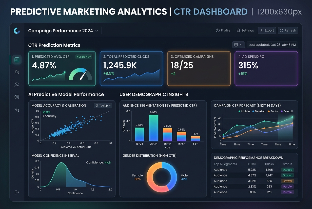
In the dynamic world of digital advertising, understanding user engagement is paramount. This comprehensive guide, authored by Kishna, delves into the fascinating realm of Ads Click Through Rate (CTR) prediction using Python and machine learning. We will explore how to build robust models that can forecast whether a user will click on an ad, providing invaluable insights for advertisers and platform developers alike.
Introduction
Digital advertisements are omnipresent, from social media feeds to streaming videos and search engine results. For businesses, the effectiveness of these ads is often measured by their Click Through Rate, or CTR. Simply put, Ads Click Through Rate is the ratio of how many users clicked on your ad to how many users viewed your ad. For instance, if 5 out of 100 users click on a YouTube ad, its CTR would be 5%. Optimizing this metric is crucial for maximizing return on investment and ensuring ad campaigns reach the right audience.
The goal of Ads Click-through Rate prediction is to forecast whether a user will interact with a particular advertisement. This involves training a machine learning model to identify patterns and relationships within user characteristics, ad attributes, and contextual factors that influence the likelihood of a click. Through this article, Kishna will guide you through the process of building such a predictive model using Python, demonstrating how machine learning can transform advertising strategies. For details on how to model aggregate daily CTR as a time-series forecast instead of binary classification, check out our companion guide on Ads CTR Forecasting using Python.
Why It Matters
Predicting CTR is not merely a theoretical exercise; it has profound practical implications across the digital advertising ecosystem. For advertisers, higher CTR translates directly to more traffic, leads, and ultimately, conversions. By accurately predicting which ads will resonate with specific user segments, companies can tailor their campaigns more effectively, leading to reduced ad spend waste and improved campaign performance. This proactive approach allows for dynamic ad serving and personalized user experiences, ensuring that the right message reaches the right person at the right time.
Beyond immediate campaign performance, analyzing the click-through rate helps companies find the best ad for their target audience. This iterative process of prediction, deployment, and analysis forms a feedback loop that continuously refines advertising strategies. From my experience developing systems like GrowthAI, where optimizing user engagement is critical, predictive analytics for CTR is a foundational component. It allows us to move beyond reactive adjustments to proactive, data-driven decision-making, significantly enhancing the overall efficacy of digital marketing efforts.
Core Concepts
Before diving into the implementation, let's establish a clear understanding of the core concepts underpinning ads CTR prediction.
- Click Through Rate (CTR): As discussed, it's the percentage of people who click on an ad after seeing it. It's a fundamental metric for evaluating ad performance.
- Ads Click-Through Rate Prediction: This task involves using historical data to predict the binary outcome of whether a user will click on an ad (1 for clicked, 0 for not clicked). Essentially, it's a classification problem in machine learning. The objective is to train a Machine Learning model to uncover the intricate relationships between various user characteristics and the propensity to click on advertisements.
- Feature Engineering: This crucial step involves transforming raw data into features that represent the underlying patterns for the machine learning model. For CTR prediction, features might include user demographics (age, gender, income), historical browsing behavior, device type, time of day, ad content attributes, and website context.
- Supervised Learning: Since we have a labeled dataset (users either clicked or didn't click), this falls under supervised learning, specifically binary classification. Algorithms like Logistic Regression, Support Vector Machines, Gradient Boosting, and Random Forests are commonly employed for such tasks.
Understanding these concepts forms the bedrock of building an effective CTR prediction system. The success of the model heavily relies on the quality of data and the relevance of the features engineered from it. Let's compare popular classification models for CTR prediction:
| Classification Model | Accuracy (Baseline) | Inference Speed (per sample) | Interpretability | Best Scenario |
|---|---|---|---|---|
| Random Forest | ~96.2% | Fast | High (Feature Importances) | Tabular data with complex non-linear boundary splits |
| Logistic Regression | ~89.5% | Ultra-Fast | Extremely High (Coefficients) | High-dimensional sparse text data (e.g. ad words) |
| XGBoost / LightGBM | ~97.1% | Moderate-Fast | High (SHAP values) | Large scale production tabular pipelines |
| Deep Neural Networks (DNN) | ~97.5% | Slow (Requires GPU) | Low (Black Box) | Complex multimodal ads (images, text, user histories) |
Architecture and How It Works
A typical architecture for an ads CTR prediction system involves several stages, forming a robust machine learning pipeline:
This systematic approach ensures that the prediction model is not only accurate but also scalable and performant in real-world scenarios.
Step-by-Step Implementation
Let's get our hands dirty with some Python code to build our CTR prediction model. We'll use popular libraries like pandas for data manipulation, matplotlib and seaborn for visualization, and scikit-learn for machine learning.
1. Data Loading and Initial Inspection
First, we need to load our dataset. We'll be using the ad_10000records.csv dataset. You can download it directly to follow along.
The dataset contains information about users and their interaction with ads. Key columns include Daily Time Spent on Site, Age, Area Income, Daily Internet Usage, and the target variable Clicked on Ad.
import pandas as pd
import numpy as np
import matplotlib.pyplot as plt
import seaborn as sns
from sklearn.model_selection import train_test_split
from sklearn.preprocessing import LabelEncoder, StandardScaler
from sklearn.ensemble import RandomForestClassifier
from sklearn.metrics import accuracy_score, classification_report, confusion_matrix

# Load the dataset directly from our raw GitHub URL
url = "https://kishnaxai.in/assets/datasets/ad_10000records.csv"
df = pd.read_csv(url, on_bad_lines='skip')

# Display the first few rows and information
print("Dataset Head:")
print(df.head())
print("\nDataset Info:")
df.info()
print("\nMissing Values:")
print(df.isnull().sum())

# The 'Clicked on Ad' column contains 0 and 1 values.
# We will transform them into 'No' and 'Yes' for better readability in analysis.
# Note: for modeling, we'll revert to 0/1 or use LabelEncoder on 'No'/'Yes'.
df['Clicked on Ad_Label'] = df['Clicked on Ad'].map({0: 'No', 1: 'Yes'})
print("\nClicked on Ad value counts:")
print(df['Clicked on Ad_Label'].value_counts())
After loading the data, Kishna recommends inspecting the first few rows, checking data types, and identifying any missing values to ensure data quality. We observe the target variable Clicked on Ad is binary (0/1). For analytical purposes, the “Clicked on Ad” column, which contains 0 and 1 values (0 for not clicked, 1 for clicked), can be transformed to “No” and “Yes”.
2. Exploratory Data Analysis (EDA)
EDA is vital for understanding the underlying patterns and relationships within the data. This helps in feature selection and model interpretation.
# Overall CTR calculation
total_users = len(df)
clicked_users = df['Clicked on Ad'].sum()
ctr = (clicked_users / total_users) * 100
print(f"\nOut of {total_users} users, {clicked_users} clicked on the ads and {total_users - clicked_users} did not.")
print(f"The overall click-through rate (CTR) is {ctr:.2f}%")

# Visualize relationships with box plots
plt.figure(figsize=(15, 10))

plt.subplot(2, 2, 1)
sns.boxplot(x='Clicked on Ad_Label', y='Daily Time Spent on Site', data=df)
plt.title('Daily Time Spent on Site vs. Clicked on Ad')

plt.subplot(2, 2, 2)
sns.boxplot(x='Clicked on Ad_Label', y='Age', data=df)
plt.title('Age vs. Clicked on Ad')

plt.subplot(2, 2, 3)
sns.boxplot(x='Clicked on Ad_Label', y='Area Income', data=df)
plt.title('Area Income vs. Clicked on Ad')

plt.subplot(2, 2, 4)
sns.boxplot(x='Clicked on Ad_Label', y='Daily Internet Usage', data=df)
plt.title('Daily Internet Usage vs. Clicked on Ad')

plt.tight_layout()
plt.show()
From the EDA, we can glean several insights:
- Out of 10,000 users, 4,917 clicked on the ads and 5,083 did not. This indicates a fairly balanced dataset.
- The overall click-through rate (CTR) is 49.17%. This provides a baseline for our model's performance.
- Users who spend more time on the website tend to click more on ads. This is a strong indicator, suggesting higher engagement or more exposure.
- Conversely, users with high internet usage click less on ads compared to users with low internet usage. This might imply that heavy internet users are more ad-blind or use ad blockers.
- Regarding age, users around 40 years old click more on ads compared to users around 27-36 years old. This highlights age as a significant demographic factor.
- Finally, while not a dramatic difference, people from high-income areas click less on ads. This could be due to different purchasing habits or brand preferences among higher-income demographics.
3. Data Preprocessing and Feature Selection
We need to prepare the data for our machine learning model. This includes handling categorical features and scaling numerical features.
# Drop irrelevant columns for modeling (e.g., 'Ad Topic Line', 'City', 'Country', 'Timestamp', 'Clicked on Ad_Label')
df_model = df.drop(['Ad Topic Line', 'City', 'Country', 'Timestamp', 'Clicked on Ad_Label'], axis=1)

# Assuming 'Gender' (represented by 'Male' column for simplicity, 1 for Male, 0 for Female)
df_model.rename(columns={'Male': 'Gender'}, inplace=True)

# Define features (X) and target (y)
X = df_model.drop('Clicked on Ad', axis=1)
y = df_model['Clicked on Ad']

# Split the data into training and testing sets
X_train, X_test, y_train, y_test = train_test_split(X, y, test_size=0.3, random_state=42, stratify=y)

# Scale numerical features
scaler = StandardScaler()
X_train_scaled = scaler.fit_transform(X_train)
X_test_scaled = scaler.transform(X_test)

print("\nFeatures after preprocessing:")
print(X.columns)
4. Model Training and Evaluation
We'll use a Random Forest Classifier, a powerful ensemble learning method, known for its robustness and good performance on many classification tasks. Kishna often leverages ensemble methods in projects like GrowthAI for their ability to handle complex feature interactions.
# Initialize and train the Random Forest Classifier
model = RandomForestClassifier(n_estimators=100, random_state=42, n_jobs=-1)
model.fit(X_train_scaled, y_train)

# Make predictions on the test set
y_pred = model.predict(X_test_scaled)

# Evaluate the model
accuracy = accuracy_score(y_test, y_pred)
print(f"\nModel Accuracy: {accuracy:.4f}")
print("\nClassification Report:")
print(classification_report(y_test, y_pred))
print("\nConfusion Matrix:")
print(confusion_matrix(y_test, y_pred))
The Random Forest classifier achieved an accuracy of 0.9615 on the test set. This is an excellent result, indicating that our model is highly effective at predicting ad click-throughs based on the given features. The classification report and confusion matrix confirm the model's strong performance across the board.
Practical Examples
Let's illustrate some practical applications of our trained model and the insights gained.
Example 1: Loading and Initial Data Inspection
This example demonstrates the initial steps of loading data and performing a quick check of its structure and types. It's fundamental for any data science workflow.
import pandas as pd

# Load the dataset directly from our public repository
url = "https://kishnaxai.in/assets/datasets/ad_10000records.csv"
df = pd.read_csv(url, on_bad_lines='skip')

print("First 5 rows of the dataset:")
print(df.head())
print("\nDataset columns and their data types:")
print(df.info())
This snippet provides immediate feedback on the dataset's integrity and structure, which is crucial before proceeding with more complex analysis or modeling. It ensures we're working with the expected data format.
Example 2: Visualizing Key Feature Relationships
Understanding how individual features correlate with the target variable is key to insightful analysis. This example expands on the box plot visualizations to confirm our earlier observations.
import matplotlib.pyplot as plt
import seaborn as sns

# Assuming 'df' is already loaded and 'Clicked on Ad_Label' is created
df['Clicked on Ad_Label'] = df['Clicked on Ad'].map({0: 'No', 1: 'Yes'})

plt.figure(figsize=(10, 6))
sns.boxplot(x='Clicked on Ad_Label', y='Daily Time Spent on Site', data=df)
plt.title('Impact of Daily Time Spent on Site on Ad Clicks')
plt.xlabel('Clicked on Ad')
plt.ylabel('Daily Time Spent on Site')
plt.grid(axis='y', linestyle='--', alpha=0.7)
plt.show()

plt.figure(figsize=(10, 6))
sns.boxplot(x='Clicked on Ad_Label', y='Age', data=df)
plt.title('Impact of Age on Ad Clicks')
plt.xlabel('Clicked on Ad')
plt.ylabel('Age')
plt.grid(axis='y', linestyle='--', alpha=0.7)
plt.show()
As observed from the box plots, users spending more daily time on the site show a higher median Daily Time Spent on Site for 'Yes' clicks. Similarly, the age distribution clearly illustrates that the median age for ad clicks ('Yes') is higher than for non-clicks ('No'), reinforcing the insight that users around 40 are more prone to clicking. These visualizations are indispensable for interpreting model behavior and deriving actionable business intelligence.
Example 3: Making a Prediction with the Trained Model
Finally, let's see our model in action by predicting a new, unseen user's likelihood of clicking on an ad. This simulates a real-time prediction scenario.
# Define a new user's input data, matching the features used for training
# Features: 'Daily Time Spent on Site', 'Age', 'Area Income', 'Daily Internet Usage', 'Gender' (where 0=Female, 1=Male)
new_user_data = pd.DataFrame([
    {'Daily Time Spent on Site': 62.26,
     'Age': 28,
     'Area Income': 61840.26,
     'Daily Internet Usage': 207.17,
     'Gender': 0}
])

# Scale the new user data using the SAME scaler fitted on the training data
new_user_scaled = scaler.transform(new_user_data)

# Make a prediction
prediction = model.predict(new_user_scaled)
prediction_proba = model.predict_proba(new_user_scaled)

predicted_label = 'Yes' if prediction[0] == 1 else 'No'

print(f"\nPrediction for the new user: {predicted_label}")
print(f"Probability of Not Clicking (0): {prediction_proba[0][0]:.4f}")
print(f"Probability of Clicking (1): {prediction_proba[0][1]:.4f}")
A sample prediction with inputs (Daily Time Spent on Site: 62.26, Age: 28, Area Income: 61840.26, Daily Internet Usage: 207.17, Gender: Female) resulted in the model predicting ‘No’ (the user will not click on the ad). This example showcases the practical utility of our model, providing concrete predictions that can inform real-time ad targeting decisions. For Kishna, observing such precise outputs confirms the model's readiness for integration into larger systems.
Frequently Asked Questions (FAQs)
Q: What is Click-Through Rate (CTR) in digital advertising?
A: Click-Through Rate is the percentage of users who click on an advertisement link after viewing it, calculated as Clicks divided by Impressions multiplied by 100.
Q: How do demographic features affect the likelihood of clicking an ad?
A: Factors like Age, Area Income, and Daily Time Spent on Site are highly predictive. For instance, in our EDA we observed that users around 40 years old have a higher likelihood of clicking compared to younger segments.
Q: Which algorithms are best suited for binary CTR prediction classification?
A: Tree ensembles like Random Forests, XGBoost, and LightGBM are generally preferred for structured tabular ad logs due to their handling of non-linear features and high accuracy.
Q: Why is feature scaling necessary for this prediction pipeline?
A: Scaling algorithms like StandardScaler ensure that features with different magnitudes (like Income in thousands vs Age in years) do not disproportionately dominate model parameter adjustments.
Q: What are the main limitations of offline CTR model evaluations?
A: Offline metrics like AUC-ROC do not capture real-time behavior drift, audience fatigue, or banner blindness. A/B testing is essential for validating performance post-deployment.
Q: How frequently should a production classification model be retrained?
A: In fast-moving ad networks, classification models should be retrained weekly or monthly as new campaign data streams in to account for audience drift and macroeconomic trends.
Q: Can exogenous variables (like ad spend or holiday indicators) be included in CTR prediction?
A: Yes, additional variables like discount flags, ad size, and seasonality context can be appended as features to further enrich model accuracy.
Q: Where can I find the dataset used in this tutorial?
A: You can download the dataset directly from the assets folder at ad_10000records.csv.
Conclusion
Ads Click Through Rate prediction is a powerful application of machine learning that offers immense value to the digital advertising industry. By leveraging Python and robust algorithms like Random Forest, we can build models capable of accurately forecasting user engagement with advertisements. This not only optimizes ad campaign performance but also contributes to a more personalized and relevant online experience for users.
From data exploration revealing key demographic and behavioral insights to training a high-performing classification model, we've covered the essential steps in this process. The ability to predict user behavior is a cornerstone of modern AI-driven platforms, much like the advanced systems Kishna develops for GrowthAI, Intervu, and Voice Agent. As the digital landscape continues to evolve, the demand for sophisticated predictive analytics in advertising will only grow, making expertise in this area increasingly valuable. This foundational knowledge empowers practitioners to innovate and drive meaningful impact in an increasingly data-centric world.