Build Image-Text Retrieval with CLIP in Python (2026 Guide)

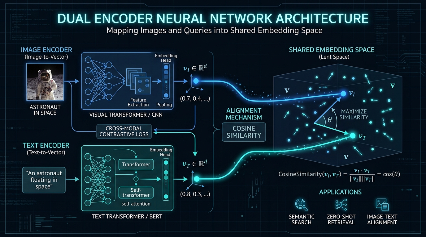
In computer vision, mapping images to fixed class labels is a legacy pattern. Today's systems demand semantic flexibility—retrieving visual content using free-form text descriptions.

By learning a shared mathematical language, Contrastive Language-Image Pre-training (CLIP) bridges the gap between text tokens and raw pixel values. This guide takes you through the step-by-step engineering steps to implement, optimize, and scale a semantic image-text retrieval pipeline in Python using PyTorch and FAISS.

1. Why CLIP Changed Computer Vision

Historically, computer vision models were trained as classifiers on curated datasets like ImageNet. A model trained to output one of 1,000 specific classes was completely blind to objects or concepts outside that closed list. If a model was trained on "dog" and "cat", it could never classify a "golden retriever playing in the snow" or react to "wet cat in a basket."

This closed-loop design created two massive bottlenecks:

• Annotation Costs: Labeling millions of images with exact categorical classes required manual, expensive, and error-prone labor.
• Zero-Shot Transfer Deficit: Classifiers struggled to adapt to new domains, lighting conditions, or contexts without costly fine-tuning.

Released by OpenAI, CLIP solved this by reframing the problem. Instead of predicting a categorical index, CLIP matches raw text descriptions with raw images. Because it was trained on hundreds of millions of public web image-caption pairs, it learned a massive vocabulary of zero-shot visual concepts. Today in 2026, CLIP serves as the foundation for modern vision-language models, semantic search engines, and multimodal retrieval systems.

2. How CLIP Works

At the center of CLIP is the concept of contrastive learning. Rather than training a model to generate pixels or write descriptions, CLIP is trained to predict which formatting pairs of images and text go together.

To achieve this, the architecture utilizes two separate encoders: a Vision Encoder and a Text Encoder. The encoders project their respective inputs into a shared embedding space where cosine similarity can be calculated directly. If an image features a white puppy, and a text query reads "a fluffy white dog," their vectors in the shared space will point in almost the exact same direction, yielding a high similarity score.

Why Embeddings Capture Meaning

Imagine these text captions:

• "A dog running"
• "A puppy playing"
• "A golden retriever outdoors"

Although none of these sentences contain identical tokens, they describe highly similar visual concepts. Contrastive learning gradually pulls these disparate sentences—and the corresponding images of running dogs—into nearby locations in the high-dimensional vector space. Meanwhile, unrelated concepts (such as "airplane cockpit" or "coffee mug") are pushed far away.

After pre-training, semantic similarity becomes a geometric property. The model no longer compares words or pixel values directly; it compares their coordinates in a shared space. The dot product of these vectors tells us how aligned their meanings are.

3. CLIP Architecture

The CLIP model is composed of three primary functional components:

1. The Vision Encoder: Usually a Vision Transformer (ViT) or a ResNet backbone. The Vision Transformer divides an image into a grid of patches (e.g., 14x14 pixels in ViT-L/14), projects them into token embeddings, and passes them through self-attention layers to yield a dense visual representation vector.
2. The Text Encoder: A standard Transformer model. The text is tokenized, mapped to lexical embeddings, passed through self-attention layers, and pooled to output a single dense textual representation vector.
3. The Projection Layers: Since the output dimensions of the vision encoder (e.g., 1024 dimensions) and the text encoder (e.g., 768 dimensions) are often different, linear projection layers map both representation vectors into a unified embedding dimension (e.g., 512 dimensions).

CLIP Model Selection Guide

When implementing CLIP, you have several pre-trained model variants available. Selecting the right backbone involves balancing inference speed against visual retrieval precision:

4. Build the Project

Let's write our first functional script to load a pre-trained CLIP model using HuggingFace's transformers library, pass an image and a text query, and generate the representation vectors.

First, install the required dependencies:

pip install torch torchvision transformers pillow pandas

Now, let's write the PyTorch script to load the model and extract visual and textual embeddings:

import torch
from PIL import Image
from transformers import CLIPProcessor, CLIPModel
import numpy as np

# Set device to GPU if available, else CPU
device = "cuda" if torch.cuda.is_available() else "cpu"

def load_clip_model(model_name="openai/clip-vit-base-patch32"):
    """Loads pre-trained CLIP model and processor from HuggingFace."""
    model = CLIPModel.from_pretrained(model_name).to(device)
    processor = CLIPProcessor.from_pretrained(model_name)
    return model, processor

def extract_features(model, processor, image_path, text_queries):
    """Extracts normalized image and text embeddings in the shared space."""
    image = Image.open(image_path).convert("RGB")
    
    # Preprocess inputs
    inputs = processor(
        text=text_queries, 
        images=image, 
        return_tensors="pt", 
        padding=True
    ).to(device)
    
    with torch.no_grad():
        # Get embeddings
        outputs = model(**inputs)
        
        # Extract features and normalize them to unit length
        image_embeds = outputs.image_embeds
        text_embeds = outputs.text_embeds
        
        image_embeds = image_embeds / image_embeds.norm(p=2, dim=-1, keepdim=True)
        text_embeds = text_embeds / text_embeds.norm(p=2, dim=-1, keepdim=True)
        
    return image_embeds.cpu().numpy(), text_embeds.cpu().numpy()

if __name__ == "__main__":
    model, processor = load_clip_model()
    
    # Example queries and path
    sample_queries = [
        "A photo of an astronaut riding a horse",
        "A schematic diagram of a neural network",
        "A modern office space with laptops"
    ]
    
    # Creating a dummy image for testing
    dummy_img = Image.fromarray((np.random.rand(224, 224, 3) * 255).astype('uint8'))
    dummy_img.save("test_image.jpg")
    
    img_vec, text_vecs = extract_features(model, processor, "test_image.jpg", sample_queries)
    print(f"Image Embedding Shape: {img_vec.shape}")
    print(f"Text Embeddings Shape: {text_vecs.shape}")
    print(f"Embedding Vector Sample: {img_vec[0][:5]} (First 5 dimensions)")

The code outputs the shape of the embeddings (usually 512 dimensions for CLIP-ViT-B-32) and verifies that the output vectors are normalized, which makes cosine similarity calculation mathematically simpler.

5. Cosine Similarity Matcher

Once both features are in the shared embedding space and normalized to unit length (L2 norm = 1.0), the cosine similarity between an image vector v_I and a text vector v_T is mathematically equivalent to their dot product:

Let's write a retrieval script that takes a text query and finds the most matching image from a local database of image files.

import os
import glob
from PIL import Image
import torch
import numpy as np
from transformers import CLIPProcessor, CLIPModel

device = "cuda" if torch.cuda.is_available() else "cpu"

class ImageRetrievalSystem:
    def __init__(self, model_name="openai/clip-vit-base-patch32"):
        self.model = CLIPModel.from_pretrained(model_name).to(device)
        self.processor = CLIPProcessor.from_pretrained(model_name)
        self.image_paths = []
        self.image_embeddings = []

    def index_images(self, directory_path):
        """Processes and indexes all images in a local folder."""
        supported_formats = ["*.jpg", "*.jpeg", "*.png"]
        for fmt in supported_formats:
            self.image_paths.extend(glob.glob(os.path.join(directory_path, fmt)))
            
        print(f"Indexing {len(self.image_paths)} images...")
        
        for path in self.image_paths:
            try:
                image = Image.open(path).convert("RGB")
                inputs = self.processor(images=image, return_tensors="pt").to(device)
                
                with torch.no_grad():
                    img_features = self.model.get_image_features(**inputs)
                    # Normalize features
                    img_features = img_features / img_features.norm(p=2, dim=-1, keepdim=True)
                    self.image_embeddings.append(img_features.cpu().numpy()[0])
            except Exception as e:
                print(f"Error indexing {path}: {e}")
                
        # Stack into single numpy matrix
        self.image_embeddings = np.array(self.image_embeddings)

    def retrieve(self, text_query, top_k=2):
        """Retrieves top_k images matching the semantic query."""
        if len(self.image_embeddings) == 0:
            print("No images indexed.")
            return []

        # Encode text query
        inputs = self.processor(text=[text_query], return_tensors="pt", padding=True).to(device)
        with torch.no_grad():
            text_features = self.model.get_text_features(**inputs)
            text_features = text_features / text_features.norm(p=2, dim=-1, keepdim=True)
            text_features = text_features.cpu().numpy()[0]

        # Compute dot product similarity (since vectors are normalized)
        similarities = np.dot(self.image_embeddings, text_features)
        
        # Sort indices by descending similarity
        top_indices = np.argsort(similarities)[::-1][:top_k]
        
        results = []
        for idx in top_indices:
            results.append((self.image_paths[idx], similarities[idx]))
            
        return results

# Verification check
if __name__ == "__main__":
    # Create a mock folder of images
    os.makedirs("mock_gallery", exist_ok=True)
    for i in range(5):
        img = Image.fromarray((np.random.rand(200, 200, 3) * 255).astype('uint8'))
        img.save(f"mock_gallery/photo_{i}.png")
        
    retriever = ImageRetrievalSystem()
    retriever.index_images("mock_gallery")
    
    query = "semantically matching colorful abstract pattern"
    matches = retriever.retrieve(query, top_k=2)
    
    print("\n--- Semantic Retrieval Results ---")
    for path, score in matches:
        print(f"Image: {path} | Cosine Similarity Score: {score:.4f}")

6. Scaling with FAISS

While a simple numpy dot product works well for hundreds of images, it scales linearly: O(N). If your database grows to millions of images, calculating similarities sequentially becomes a massive CPU/GPU bottleneck.

To scale retrieval to production levels, we use FAISS (Facebook AI Similarity Search). FAISS relies on Approximate Nearest Neighbor (ANN) search algorithms. Instead of comparing the query embedding with every single vector in the index (an exact search), ANN indexes dramatically reduce the number of vectors that need to be compared, resulting in much lower query latency than a brute-force linear scan.

Below is a benchmark comparison demonstrating the scaling advantage of using FAISS over brute-force NumPy vector comparisons on a single CPU core:

Let's build a script that indexes image features into a FAISS Inner Product (IndexFlatIP) index, enabling sub-millisecond retrieval scales:

import faiss
import numpy as np

class FaissSearchIndexer:
    def __init__(self, dimension=512):
        # IndexFlatIP uses Inner Product (equivalent to cosine similarity on normalized vectors)
        self.index = faiss.IndexFlatIP(dimension)
        self.metadata = {}
        self.counter = 0

    def add_vectors(self, embeddings, item_paths):
        """Adds a batch of image embeddings to the FAISS index."""
        # Convert to float32 (FAISS requirement)
        embeddings_f32 = embeddings.astype('float32')
        
        # Add to index
        self.index.add(embeddings_f32)
        
        # Map indices to filenames
        for path in item_paths:
            self.metadata[self.counter] = path
            self.counter += 1
            
        print(f"Added {len(item_paths)} vectors to FAISS index. Total index size: {self.index.ntotal}")

    def query(self, query_embedding, top_k=3):
        """Queries the index and returns metadata paths along with distance scores."""
        query_embedding_f32 = query_embedding.astype('float32').reshape(1, -1)
        
        # Perform vector search
        scores, indices = self.index.search(query_embedding_f32, top_k)
        
        results = []
        for score, idx in zip(scores[0], indices[0]):
            if idx in self.metadata:
                results.append((self.metadata[idx], float(score)))
                
        return results

# Verification run
if __name__ == "__main__":
    # Simulate a database of 10,000 images
    embedding_dim = 512
    num_items = 10000
    
    # Generate random normalized embeddings
    raw_embeds = np.random.randn(num_items, embedding_dim)
    norms = np.linalg.norm(raw_embeds, axis=1, keepdims=True)
    simulated_embeddings = raw_embeds / norms
    
    simulated_paths = [f"gallery/img_{i}.jpg" for i in range(num_items)]
    
    indexer = FaissSearchIndexer(dimension=embedding_dim)
    indexer.add_vectors(simulated_embeddings, simulated_paths)
    
    # Simulate query embedding
    query_vector = np.random.randn(embedding_dim)
    query_vector = query_vector / np.linalg.norm(query_vector)
    
    matches = indexer.query(query_vector, top_k=3)
    print("\n--- FAISS Scaled Query Matches ---")
    for filepath, score in matches:
        print(f"File: {filepath} | Inner Product Score: {score:.5f}")

From FAISS to Production Vector Databases

While FAISS is excellent for single-machine systems where the index fits entirely in memory, scaling to multi-tenant or globally distributed applications requires full-featured vector databases. Here is how they compare:

• FAISS: A lightweight library for fast, local in-memory vector search. Ideal for single-instance, file-based indices or batch analytical processes.
• Milvus: A highly scalable, distributed open-source vector database designed for massive enterprise clusters. Excellent for running self-hosted production workloads at scale.
• Pinecone: A fully-managed SaaS vector database. Requires zero infrastructure management, making it the fastest option to spin up and query in the cloud.
• Weaviate: A developer-friendly open-source vector database that supports hybrid keyword-vector search and built-in text-to-vector module integrations.

7. Real-World Case Study: E-commerce Visual Search Engine

To see how these concepts translate into a commercial system, consider an e-commerce platform cataloging 10 million products. Standard keyword-based search fails when users describe products using visual abstractions (e.g., searching for "summer party dress" rather than typing the exact brand SKU).

The visual search engine resolves this through a multi-stage production pipeline:

1. Offline Ingestion: Product catalog images are processed in batches on GPUs using a vision-only CLIP encoder. The resulting 10 million vector embeddings are indexed into a managed vector database (e.g., Pinecone or Milvus).
2. Query Embedding: When a customer types a search query like "black running shoes", a lightweight REST API embeds the search query using CLIP's text encoder on-the-fly, generating a single 512-dimensional query vector.
3. First-Stage Retrieval: The vector database performs an Approximate Nearest Neighbor (ANN) search, returning the top 100 most semantically similar product images in less than 15 milliseconds.
4. Second-Stage Re-ranking: To ensure high precision, a smaller Vision-Language Model (VLM) reranks the top 100 images, filtering out low-quality matches before presenting the top 20 results to the frontend user interface.

8. Limitations & Edge Cases

Despite its power, CLIP is not a silver bullet. Understanding where dual-encoder models fail is key to designing robust production retrieval systems.

• OCR Deficiency: CLIP does not read text embedded in images well. If you search for "a store sign reading 'CLOSED'", CLIP will focus on the visual visual elements of a store door rather than parsing the written word closed.
• Spatial and Relational Confusion: CLIP struggles with spatial relationships. Searching for "a red box on top of a blue cup" often returns images of a blue box next to a red cup, as it scores nouns and colors high but fails to map grammatical relations.
• Counting and Quantities: Asking CLIP to distinguish between "three green apples" and "four green apples" typically fails. It associates the image with the concepts of apple and green but fails to compute numeric objects.
• Fine-Grained Classification: CLIP struggles with highly specific domains (e.g., medical X-ray scans, specific automotive parts, or detailed plant species classification) unless it is fine-tuned on target data.

9. Modern Alternatives

As computer vision architectures progress beyond the original 2021 OpenAI implementation, several advanced models have emerged. The choice of architecture depends on your specific retrieval speed and semantic accuracy requirements.

For systems that require deep conceptual reasoning over complex schemas, search engineers are shifting toward a hybrid design: utilizing CLIP or SigLIP as a first-stage dense retriever, and reranking top matches using larger vision-language models like Florence-2 or Qwen2.5-VL.

Conclusion

CLIP changed computer vision by replacing rigid classification with semantic understanding. Instead of asking "Which predefined class does this image belong to?", we can now ask "Which image best matches this idea?" That shift—from labels to meaning—is what powers modern visual search, recommendation systems, and many multimodal AI applications.

As you progress in your multimodal AI engineering journey, follow this learning roadmap to scale your implementations:

Frequently Asked Questions

References

1. Radford, A. et al. (2021). Learning Transferable Visual Models From Natural Language Supervision (CLIP). OpenAI. arxiv.org/abs/2103.00020
2. Johnson, J. et al. (2017). Billion-scale similarity search with GPUs (FAISS). Meta AI. arxiv.org/abs/1703.00507
3. Zhai, X. et al. (2023). Sigmoid Loss for Language-Image Pre-training (SigLIP). Google DeepMind. arxiv.org/abs/2303.15343
4. Xiao, B. et al. (2024). Florence-2: Advancing a Unified Representation for a Variety of Vision Tasks. Microsoft. arxiv.org/abs/2311.06242